Introduction

Picture this, you are a developer from Nigeria attending Google IO Extended at Strathmore University in Nairobi, Kenya as a speaker. Undoubtedly some of the questions you'll ask yourself in preparation for your journey will be:

• Where is Strathmore University?
• How do I get there? Uber, Taxi, Matatu?
• When is my session beginning?
• In which room/venue will the session be?
• How much time do I have?
• Will my presentation fit within the time allocated, or will I need to make changes?
• Which attendee demographic will I be dealing with? Will there be kids, novices, or pros? Will I need to dumb down my presentation a notch? Among others.

Unknown to you, as you were figuring out the answers to these questions, you just did an Exploratory Data Analysis (EDA). You explored (albeit online), prepared beforehand, understood what to expect, and ultimately improved your delivery on a material day.

Similarly, before embarking on any machine learning project, it is imperative to perform an EDA to ensure that the data at hand is ready for modeling. EDA helps you look at the data to identify obvious errors quickly, understand data patterns within the dataset and unearth relationships/ correlations among variables.

Moreover, it will guide you in detecting outliers and strange events in the data. Think of it like a detective finding puzzle pieces in the data.

In the absence of an EDA, you're basically walking into the data blind as a bat. The chances are high your machine learning model will suffer inaccuracies, and the algorithms might not even work altogether.

What is EDA?

"Exploratory data analysis is an attitude, a state of flexibility, a willingness to look for those things that we believe are not there, as well as those that we believe to be there." John Tukey.

Exploratory Data Analysis (EDA) is a data discovery technique that often employs data visualization methods to investigate datasets and summarise their outstanding characteristics. It acts as a guide to how best to manipulate data to get the desired answers, thus making it easier to discover patterns, test a hypothesis, and spot anomalies.

In addition, performing an EDA provides you with a better understanding of data set variables and the relationships between them and guides your choice of statistical techniques to be used during model building.

How Do We Go About It?

For the following section, I will be sharing some python code snippets to help you follow along.

1. Import the data

Import the data you're working with into your IDE, be it Jupyter Notebooks or Google Colaboratory. I found Colab to be more user-friendly for writing fast code without requiring a lot of environment setup. The fact that it runs on the cloud also gives that added assurance that your code is autosaved and only a login away.

So start coding from your work desktop, go home, and continue where you left on your laptop. However, it also means no offline coding as it requires internet access to work, and files uploaded to the service only last the entirety of the session. But I digress…

dataset = pd.read_csv(r'Job_Frauds.csv', encoding="ISO-8859-1")
dataset

2. Check Your Data Types.

Remember how you needed to know the demographic of the attendees to your Google IO presentation; same case here. You will need to understand the data types you will be working with. A simple function to do this would be

dataset.info()

Output

<class 'pandas.core.frame.DataFrame'>
RangeIndex: 17880 entries, 0 to 17879
Data columns (total 16 columns):
 #   Column              Non-Null Count  Dtype 
---  ------              --------------  ----- 
 0   Job Title           17880 non-null  object
 1   Job Location        17534 non-null  object
 2   Department          6333 non-null   object
 3   Range_of_Salary     2868 non-null   object
 4   Profile             14572 non-null  object
 5   Job_Description     17879 non-null  object
 6   Requirements        15185 non-null  object
 7   Job_Benefits        10670 non-null  object
 8   Telecommunication    17880 non-null  int64 
 9   Comnpany_Logo       17880 non-null  int64 
 10  Type_of_Employment  14409 non-null  object
 11  Experience          10830 non-null  object
 12  Qualification       9775 non-null   object
 13  Type_of_Industry    12977 non-null  object
 14  Operations          11425 non-null  object
 15  Fraudulent          17880 non-null  int64 
dtypes: int64(3), object(13)
memory usage: 2.2+ MB

This further helps you see the column names in your dataset and the number of filled entries per column (non-null values). Speaking of null values, this brings us to the next step.

3. Check for Null Values

Ideally, you want to check for null values as they could vastly affect your data.

dataset.isna().sum()

Output

Job Title                 0
Job Location            346
Department            11547
Range_of_Salary       15012
Profile                3308
Job_Description           1
Requirements           2695
Job_Benefits           7210
Telecommunication          0
Comnpany_Logo             0
Type_of_Employment     3471
Experience             7050
Qualification          8105
Type_of_Industry       4903
Operations             6455
Fraudulent                0
dtype: int64

Kindly note that a lot of consideration is needed when dealing with null values. You can either omit /drop the blank entries, fill them with values of a measure of central tendency (mode, mean, median), or add custom values for each empty cell. The easiest way to eliminate them would be to delete the rows with the missing data for missing values. However, this has the downside: it could result in loss of information. Additionally, this approach works poorly when the percentage of missing values is excessive compared to the entire dataset.

If, however, you chose to drop, then you could write a function to evaluate the number of nulls as a percentage of the column entries, and, based on a predetermined value, drop those columns. Say drop all columns where the null percentage is greater than 60% of column values

nan_cols = []

for col in dataset.columns:
    nan_rate = dataset[col].isna().sum() / len(dataset)

    # display null value rate
    print(f"{col} column has {round(nan_rate, 2) * 100}% of missing values")

    # add columns with more than 60% missing values to the empty list
    if (nan_rate > 0.6).all():
        nan_cols.append(col)

# display list of columns that will be dropped
print(f"Columns {nan_cols} have more than 60% of missing values and will be dropped")
dataset = dataset.drop(columns=nan_cols)

Output

Job Title column has 0.0% of missing values.
Job Location column has 2.0% of missing values
Department column has 65.0% of missing values
Range_of_Salary column has 84.0% of missing values
Profile column has 19.0% of missing values
Job_Description column has 0.0% of missing values
Requirements column has 15.0% of missing values
Job_Benefits column has 40.0% of missing values
Telecommunication column has 0.0% of missing values
Comnpany_Logo column has 0.0% of missing values
Type_of_Employment column has 19.0% of missing values
Experience column has 39.0% of missing values
Qualification column has 45.0% of missing values
Type_of_Industry column has 27.0% of missing values
Operations column has 36.0% of missing values
The fraudulent column has 0.0% of missing values
Columns ['Department,' 'Range_of_Salary'] have more than 60% of missing values and will be dropped

4. Statistical Insights

You can generate measures of central tendency and other statistical data insights using the .describe() function. This includes information on the:

• Count
• Mean
• Quartile ranges
• Maximum
• Minimum
• Standard deviation of the data.

  dataset.describe()
  

5. Dropping Duplicate Rows

Do this to eliminate redundancies in the dataset

print(dataset.shape)
dataset = dataset.drop_duplicates()
print(dataset.shape)

Output

(17880, 16)
(17592, 16)

The number of rows in the dataset reduced to 17592 after the elimination of 288 duplicate entries

6. Column Splitting

At times, too much information per column/feature could end up making that column useless. For example, a column with "US, NY, New York" won't be beneficial to your analysis especially if you intended on doing geographical plotting visualizations. In cases such as these, splitting this column into three namely Country, State and City make more sense.

# split columns and add new columns to the dataset
dataset[['Country', 'State', 'City']] = dataset['Job Location'].str.split(',', n=2, expand=True)
# display the dataframe
dataset

Output

Country State  City
US      NY       New York

7. Data Imbalance

This mainly applies to classification problems where we have binary output, say 0 and 1. A classification data set with skewed class proportions are considered imbalanced.

dataset.Fraudulent.value_counts()

Output

0    17014
1      866
Name: Fraudulent, dtype: int64

The data above is highly imbalanced with a minority class to majority class ratio of 1:19.6. This poses a real problem for classification models as the model will spend most of its time on false examples and not learn enough from true ones. We will not dwell on imbalanced data as it is an entire topic on its own. That said, however, you could look into techniques to remedy this such as;

• Downsampling - train the model on a disproportionately low subset of the majority class
• Upweighting - Taking the factor by which you downsampled, and adding an example weight to the downsampled class equal to that.

8. Pandas Data Profiling

At this point, you're probably asking the lazy question, "Is there an easier way to get this done?" And I respect that because that exact line of questioning is what makes for a good programmer (Other than knowing how to Google of course).

In my time as a data masseur, I have found that employing pandas' data profiling function works like a charm. Get this, it summarises the dataset, generates a report structure, and renders it in HTML all in just 4 lines of code. Start by importing the required libraries

# Installing panda profiling requirements for exploratory data analysis
! pip install https://github.com/pandas-profiling/pandas-profiling/archive/master.zip

Use it

# Using panda profile to get an overview of the data
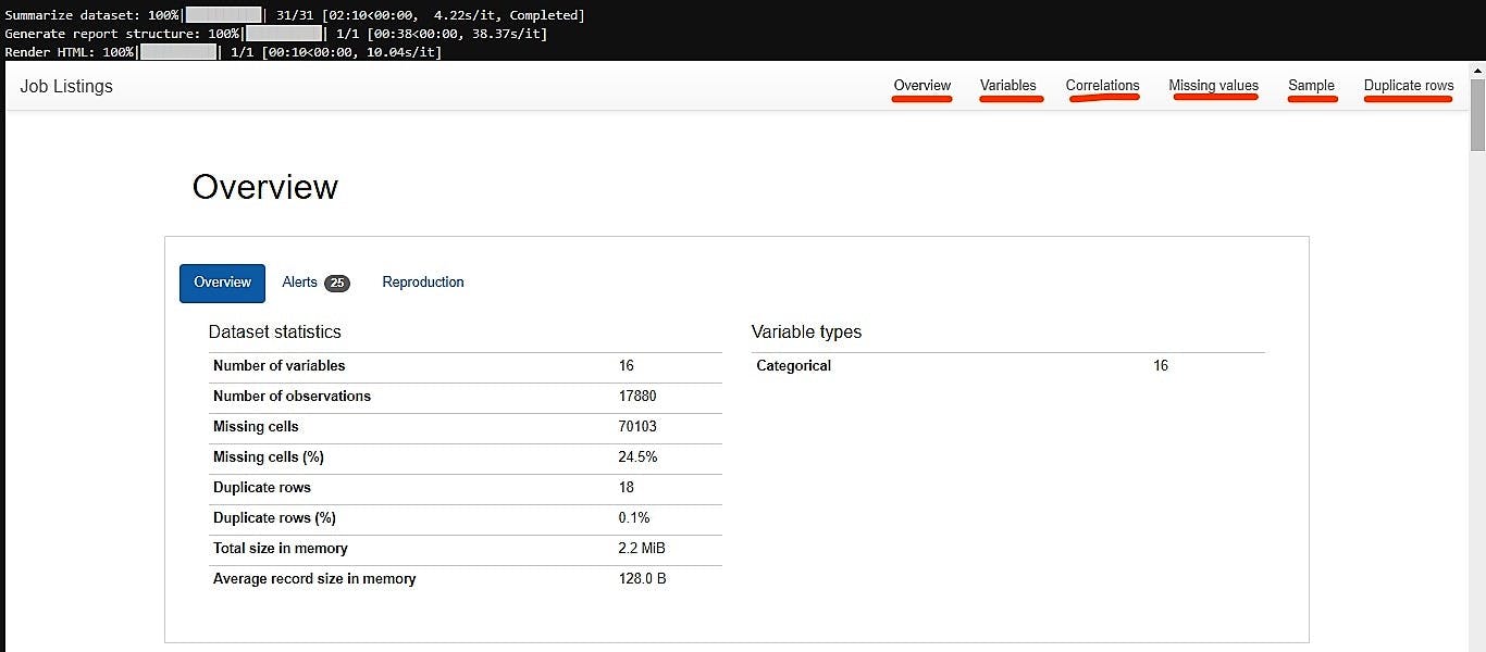
profile = ProfileReport(dataset, title="Job Listings", html={'style': {'full_width': True}}, sort=None)
profile.to_notebook_iframe()
# to save  or output the file
profile.to_file(output_file = "JobFraud.html")

The code above will; Display a descriptive overview of the data sets i.e

• the number of variables,
• observations,
• total missing cells,
• duplicate rows,
• memory used and
• the variable types.

Generate detailed analysis for each variable in the set. This is everything from;

• class distributions,
• interactions,
• correlations,
• missing values,
• samples and
• duplicated rows.

Get you a rendered HTML report that you can save for later. Output

9. Visualizations

A picture speaks a thousand words but in data, it sings in a million beautiful graphs. Visualizations breathe life into data. Transforming crowded digits into interactive plots that convey the same message or more in a fraction of the time. There exists numerous tools that come in handy when doing EDA visualizations. Some of them are seaborn, matplotlib, pandas, Plotly, and cufflinks. Some common plots used are bar plots, count plots, violin plots, histograms, and correlation matrices.

Conclusion

Needless to say, a better understanding of your data beforehand greatly improves the quality of your model's outcome. An in-depth EDA also goes a long way in improving the confidence you have with your data and could help you in formulating your hypotheses moving forward. Moreover, it will greatly reduce your time to production and make your work easier.

Some will say that's being lazy, and to that, I say, "May the lazy ones assemble". In data science, it's okay to be "lazy". It means you will always look for the fastest, easiest way to get the job done. If that's what you train your algorithms to do, then why can't you? "And that's on optimization!"

That has been it from me. See you on the next one. Be Safe. Be Kind. Peace.