


Introduction
Picture this, your sister is in the market for a used car. Being the family’s resident techie and the single point of truth for automotive information, she asks for your help in coming up with the best car at her price point. After a long time looking you come across an industry report detailing buyer purchase trends within that segment. Included in the report are the make and model, safety ratings, mileage, year of manufacture, owner’s favourite music genre, fuel efficiency, previous owner’s name etc.
Many of these probably have some effect on the price, but by how much? You go ahead and build a model to predict car prices. During your EDA you realise that the model of the car, the year of manufacture, and the mileage are pretty important determinants of a vehicle’s asking price. However, the name of the previous owner or their music taste has zero influence on the price. Further, they confuse the algorithm into finding patterns between names, music genres and the other features. Hence you decide to drop those two columns and only use the most relevant features for your model.
In doing so, you just did feature selection. You were presented with a number of distinct features to train your model on and rather than throw them all at the model you realised that some of the features would not have any predictive power for your desired label. Best case scenario, using them would only increase training time, At worst, these irrelevant features would increase model complexity, training time as well as the prediction error rates.
In this article we discuss feature selection, what it is and why even bother with it. We then delve into programming in python to show how you can perform feature selection on your dataset using three common techniques.
What is Feature Selection?
Also goes by the names Variable Selection, Attribute Selection or Variable Subset Selection. It is the process of selecting a subset of relevant features for use in model building. Feature selection works under the general premise that the dataset you are working with contains a set of features that are either redundant or irrelevant and can, as a result, be eliminated without incurring much information loss. Here, a feature is an attribute that has an impact on a problem or is useful for the problem and is mostly represented by columns.
Why bother with it?
The Curse of Dimensionality
Feature selection helps you avoid the curse of Dimensionality. Simply put, this is a problem in data mining in large data sets with many potential predictor variables. In this case, an increase in features leads to an increase in accuracy upto a certain threshold value after which increasing features leads to a decrease in model accuracy. This happens because, before a certain threshold value, your model is learning from useful information, however, as you increase the number of features past this threshold value, the model gets “confused”. The reason for this behaviour is that your model is being fed with too much information making it unable to train with the correct information i.e the introduction of noise in the data hence the decrease in accuracy. So, beyond that threshold value when the model’s accuracy starts decreasing with every subsequent increase in number of features, there arises The Curse of Dimensionality.
The law of Parsimony (Occam's Razor)
This principle states that the best explanation to a problem is that which involves the fewest possible assumptions i.e entities should not be multiplied beyond necessity. In other words, a model with fewer parameters is to be preferred. The goal of feature selection is to create a model that achieves a desired level of goodness of fit using as few explanatory variables as possible i.e a Parsimonious Model. Applied to machine learning, a model with few parameters but achieves a satisfactory level of goodness of fit should be preferred over a model that has a ton of parameters and achieves only a slightly higher level of goodness of fit.
Others
In addition to the above reasons, the following are other reasons why you should make it a habit to implement feature selection whenever possible in your data journey.
- It helps in simplifying your models and by doing so, makes them easier to interpret by the users.
- It reduces the computational cost of modelling through shorter training times. The result of which is most noticeable when dealing with enormous amounts of data.
- It helps increase the precision of the estimates that can be obtained for a given simulation hence helping you achieve variance reduction
- It reduces overfitting since less redundant data means fewer opportunities to make bad decisions based on noise.
Examples with Code
In the following section I use the Mobile Price Classification dataset from Kaggle to briefly go over how to perform feature selection using three common techniques; Univariate Selection, Feature Importance and Correlation Matrix with Heatmap. I intend to find out which among the many features in a mobile phone has the most impact on its price.
Dataset Variable Description
+----+---------------+--------------------------------------------------------------------------------------------------------------+
|    | Variable      | Description                                                                                                  |
+====+===============+==============================================================================================================+
|  0 | battery_power | Total energy a battery can store in one time measured in mAh                                                 |
+----+---------------+--------------------------------------------------------------------------------------------------------------+
|  1 | blue          | Has Bluetooth or not                                                                                         |
+----+---------------+--------------------------------------------------------------------------------------------------------------+
|  2 | clock_speed   | the speed at which microprocessor executes instructions                                                      |
+----+---------------+--------------------------------------------------------------------------------------------------------------+
|  3 | dual_sim      | Has dual sim support or not                                                                                  |
+----+---------------+--------------------------------------------------------------------------------------------------------------+
|  4 | fc            | Front Camera megapixels                                                                                      |
+----+---------------+--------------------------------------------------------------------------------------------------------------+
|  5 | four_g        | Has 4G or not                                                                                                |
+----+---------------+--------------------------------------------------------------------------------------------------------------+
|  6 | int_memory    | Internal Memory in Gigabytes                                                                                |
+----+---------------+--------------------------------------------------------------------------------------------------------------+
|  7 | mobile_wt     | Weight of mobile phone                                                                                       |
+----+---------------+--------------------------------------------------------------------------------------------------------------+
|  8 | n_cores       | Number of cores of the processor                                                                             |
+----+---------------+--------------------------------------------------------------------------------------------------------------+
|  9 | pc            | Primary Camera megapixels                                                                                    |
+----+---------------+--------------------------------------------------------------------------------------------------------------+
| 10 | px_height     | Pixel Resolution Height                                                                                      |
+----+---------------+--------------------------------------------------------------------------------------------------------------+
| 11 | px_width      | Pixel Resolution Width                                                                                           |
+----+---------------+--------------------------------------------------------------------------------------------------------------+
| 12 | ram           | Random Access Memory in MegaBytes                                                                            |
+----+---------------+--------------------------------------------------------------------------------------------------------------+
| 13 | sc_h          | Screen Height of mobile in cm                                                                                |
+----+---------------+--------------------------------------------------------------------------------------------------------------+
| 14 | sc_w          | Screen Width of mobile in cm                                                                                 |
+----+---------------+--------------------------------------------------------------------------------------------------------------+
| 15 | talk_time     | the longest time that a single battery charge will last when you are talking                                 |
+----+---------------+--------------------------------------------------------------------------------------------------------------+
| 16 | three_g       | Has 3G or not                                                                                                |
+----+---------------+--------------------------------------------------------------------------------------------------------------+
| 17 | touch_screen  | Has touch screen or not                                                                                      |
+----+---------------+--------------------------------------------------------------------------------------------------------------+
| 18 | Wifi          | Has wifi or not                                                                                              |
+----+---------------+--------------------------------------------------------------------------------------------------------------+
| 19 | price_range   | This is the target variable with a value of 0(low cost), 1(medium cost), 2(high cost) and 3(very high cost). |
+----+---------------+--------------------------------------------------------------------------------------------------------------+
Univariate Selection
We can use statistical tests to get the features with the strongest relationship with the target output. For this example we utilise the scikit-learn library sklearn.feature_selection.SelectKBest to select features according to the K highest scores.
It is also advisable to use this alongside the Chi-Square test. Since Chi-square tests measure the dependence between stochastic variables, using this function eliminates features that are most likely independent of class and therefore irrelevant for the classification.
Input
import pandas as pd
import numpy as np
from sklearn.feature_selection import SelectKBest
from sklearn.feature_selection import chi2
data = pd.read_csv("train.csv")
X = data.iloc[:,0:20]  #independent columns
y = data.iloc[:,-1]    #target column i.e price range
#apply SelectKBest class to extract top 10 best features
bestfeatures = SelectKBest(score_func=chi2, k=10)
fit = bestfeatures.fit(X,y)
dfscores = pd.DataFrame(fit.scores_)
dfcolumns = pd.DataFrame(X.columns)
#concat two dataframes for better visualization
featureScores = pd.concat([dfcolumns,dfscores],axis=1)
featureScores.columns = ['Specs','Score']  #naming the dataframe columns
print(featureScores.nlargest(10,'Score'))  #print 10 best features
Output
           Specs          Score
13            ram  931267.519053
11      px_height   17363.569536
0   battery_power   14129.866576
12       px_width    9810.586750
8       mobile_wt      95.972863
6      int_memory      89.839124
15           sc_w      16.480319
16      talk_time      13.236400
4              fc      10.135166
14           sc_h       9.614878
Analysis
Having a look at the output, we can deduce that RAM, battery power and the size of the phone (px_height and px_width) have the most impact on a phone’s price and this is the case with industry as well.
Feature Importance
The feature importance property of your model can help you get the feature importance of each variable in your dataset. The higher the score the more relevant the feature is towards your output variable.
Luckily sklearn Tree Based Classifiers has feature importance as an inbuilt class. This means we can use Extra Tree Classifier to get the top 10 features for the dataset.
Input
import pandas as pd
import numpy as np
data = pd.read_csv("train.csv")
X = data.iloc[:,0:20] #independent columns
y = data.iloc[:,-1] #target column i.e price range
from sklearn.ensemble import ExtraTreesClassifier
import matplotlib.pyplot as plt
model = ExtraTreesClassifier()
model.fit(X,y)
print(model.feature_importances_) #use inbuilt class feature_importances of tree based classifiers
#plot graph of feature importances for better visualization
feat_importances = pd.Series(model.feature_importances_, index=X.columns)
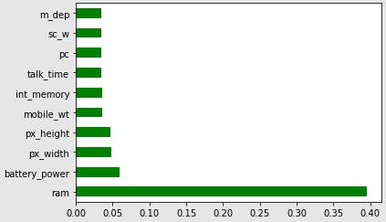
feat_importances.nlargest(10).plot(kind='barh')
plt.show()
Output
Correlation Matrix with Heatmap
This is possibly the most common of the three. Correlation shows how variables are related to each other and to the target variable and can either be positive (increase in one feature value increases the target variable) or negative (increase in one feature value decreases the target variable). A heatmap plot on the other end makes it easier to visually identify related features. We will be using the seaborn library for the plot below.
Input
import pandas as pd
import numpy as np
import seaborn as sns

data = pd.read_csv("train.csv")

X = data.iloc[:,0:20]  #independent columns
y = data.iloc[:,-1]    #target column i.e price range

#get correlations of each features in dataset
corrmat = data.corr()
top_corr_features = corrmat.index
plt.figure(figsize=(10,10))

#plot heat map
g=sns.heatmap(data[top_corr_features].corr(),annot=True,cmap="PiYG")
Output
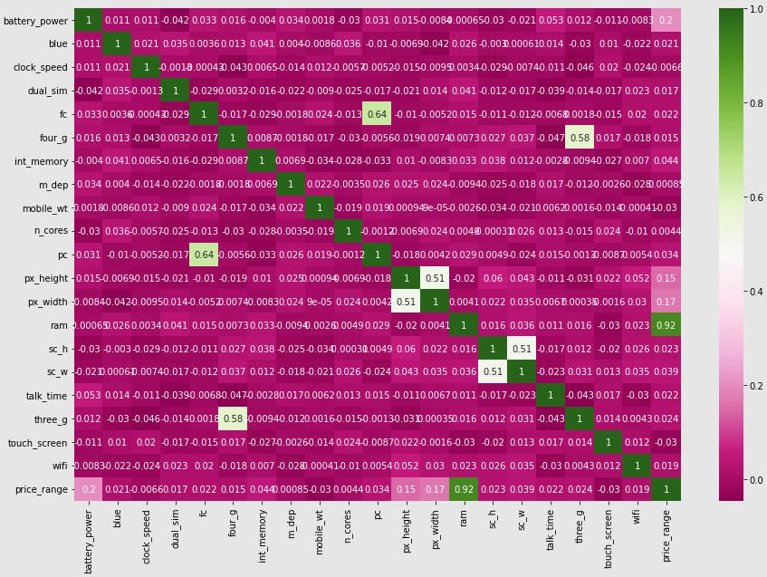
Analysis
Looking at the last column (price_range) you can clearly see how it correlates with the other features. It supports our other feature selection methods with RAM and phone size being key determinants of price.
Conclusion
In this article we have looked at feature selection and how univariate selection, feature importance and correlation matrix can help you tackle the curse of dimensionality by weeding out irrelevant features. So next time you go for hackathons and you wonder how, with the same model and computational facilities, some teams end up winning, the answer could just be Feature Selection. Also bear in mind that apart from choosing the right model for your data, you need to choose the right data to feed into your model, always striving to produce a parsimonious model.
That has been it from me. See you on the next one. Be Safe. Be Kind. Peace